A Paper Published

Chinese version (中文版): https://mp.weixin.qq.com/s/wsyNqSQVBj6GH_AF0d6Izw

Publisher’s link for this paper: https://onlinelibrary.wiley.com/doi/full/10.1002/mrm.70022

In my final year as a PhD student, I worked on something quite interesting: using the power of deep learning to predict knee joint T1rho images with incomplete physical information. To those familiar with deep learning, this might not seem like a big deal—after all, deep learning can generate lifelike images from a patch of noise. But to people in the magnetic resonance imaging (MRI) field, might don’t agree: it’s almost like throwing away MRI physics and using purely statistical experience to create images that appear physically meaningful. From my observations at the ISMRM annual meetings over the past few years, it seems the community has taken a considerable amount of time to accept this type of work.

We gave this work a very long title: Utilizing 3D fast spin echo anatomical imaging to reduce the number of contrast preparations in T1rho quantification of knee cartilage using learning-based methods. This work was led by me as the first author, with my PhD supervisor Professor Weitian Chen as the corresponding author; my fellow group member Chaoxing Huang was a major contributor.

This work was submitted to the top journal in the MRI community, Magnetic Resonance in Medicine, in February 2025, accepted in July of the same year, and officially published online a few days ago. If you don’t want to read my ramblings, you can click “Read more” at the end of the article to go directly to the paper. Thanks to the sponsorship of the university library, this paper is now Open Access, so everyone can view and download it freely here.

Background

The background of this work originates from my PhD supervisor Professor Weitian Chen’s early career experience in the industry—they hoped to achieve simultaneous high-resolution knee anatomical and T1rho imaging through a 3D fast spin echo sequence (3D FSE/TSE). This goal, it can be said, has not yet been fully realized even at the time of this paper’s publication. The main challenge is that T1rho imaging typically requires acquiring multiple (usually 4) spin-lock prepared images, which are then used to fit a signal model. One T1rho imaging method recommended by the RSNA, 3D MAPSS based on gradient echo imaging (GRE), can complete a T1rho acquisition in 5-12 minutes [1]. Although this is not slow, we believe there is still an issue: T1rho itself is an additional knee acquisition sequence. It doesn’t do anything more on its own and is an extra time burden for the entire knee scan. In contrast, the 3D FSE-based T1rho acquisition method our group has been developing long-term has image features similar to proton density (PD) at a time of spin-lock (TSL) of 0, which is similar to the clinically acquired PD-w FSE images.

Besides the sequence-related reasons, we also developed and observed the gradual maturation of deep learning-based acceleration methods for T1rho and other quantitative MRI. These acceleration methods not only include conventional k-space-based methods, such as MANTIS [2], but also many methods that fit the signal model using fewer acquired images, such as the work by this paper’s main contributor, Chaoxing Huang, on liver T1rho [3,4,5]. Based on Chaoxing’s work, we wondered if we could, based on the image similarity caused by the sequences mentioned above, replace the TSL=0 T1rho image with a PD-w image and feed it into a neural network along with a T1rho image with a non-zero TSL to predict the final T1rho quantification.

Implementation

Data

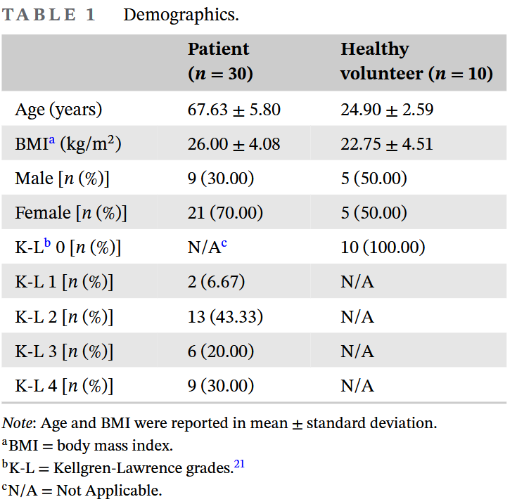
We dug out images from 30 knee osteoarthritis patients and 10 volunteers from previous projects. Because knee osteoarthritis is common in the elderly, and the volunteers were friends from around the lab, we can see that the age and BMI gaps between the two groups are quite large. At the same time, this batch of data had a majority of late-stage OA patients, and many also had cartilage perforations. But in the end, because the amount of data was too small, we had to mix all the images from the 40 participants together for use.

MRI Pulse Sequence Design

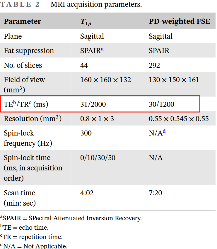
In terms of sequence design, we used the most standard 3D FSE T1rho implementation [6] and a conventional 3D FSE sequence. The image readouts for both sequences used Philips’ commercial implementation (VISTA™). The sequence parameter table above provides the TE/TR parameters for the two sequences; you can see that both are PD-weighted with a short TE and long TR. Since I’m not a sequence expert, I won’t try to show off here. For specific sequence implementation details, you can refer to the original paper and reference [6].

Image Preprocessing

Before moving on to deep learning, we also needed to perform a series of image preprocessing steps. Looking at the MRI parameters above, it’s not hard to see that these two sequences were not acquired from the same FOV (it was old data). Therefore, we first registered the two images from the same person, transforming the high-resolution PD-w FSE image to match the relatively lower-resolution T1rho image. We used the handy ANTsPy toolkit, employing a three-stage registration: rigid -> affine -> deformable (SyN, [7]), to ensure the cartilage regions were aligned as much as possible. After registration, we confirmed that the Structural Similarity Index (SSIM) within the cartilage regions reached a high level of 0.97 ± 0.01 (mean ± standard deviation). The specific registration process can be found in the supplementary material S1 of the original paper.

We had previously prepared segmentation labels for four cartilage regions (femoral, medial and lateral tibial, and patellar cartilage) on the T1rho images of this dataset. In the experiments and analysis of the main text, we will merge these four cartilage regions into a single complete cartilage region for statistical calculations. As for the metrics for the four individual cartilage regions, due to the large amount of data, we provide them in the supplementary material S3 of the original paper.

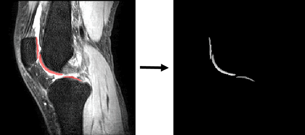
After registration, we split the 3D images into 2D slices or 1D vectors according to the experimental design. One set of 2D slices would also be masked, while the 1D vectors would only contain the pixel values within the cartilage regions. During the splitting process, we retained the relevant positional information to restore the T1rho values predicted by the neural network to their corresponding 3D spatial positions for visualization and calculation of experimental metrics.

Neural Network Design

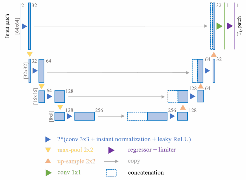
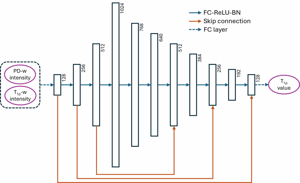
From the very beginning of the project, we didn’t intend to create a very complex neural network design. There are two reasons: first, our audience is mainly scholars in the MRI community, who may not be familiar with or approve of the advanced neural network models in the deep learning community today; second, we believe that the simpler the neural network design, the more it demonstrates the universality of our hypothesis. So in this paper, we only introduced two very simple but time-tested neural network designs: a U-Net [8] with a replaced regressor and a multi-layer perceptron (MLP, modified from [9]) with skip-connections, using 2D and 1D data respectively.

We introduced two simple tricks to the 2D U-Net to improve the model’s stability:

• Before the data is input into the model, we crop small patches of 64 × 64 pixels at random locations around the cartilage region from the original 256 × 256 pixel images. These patches then undergo multiple transformations for data augmentation. This process introduces randomness into the training data and greatly expands the actual amount of usable data, thereby improving the model’s stability and performance.
• At the end of the 2D U-Net, before the final output, we introduced a clipper. This clipper removes unreasonable T1rho value predictions (i.e., less than 10 or greater than 100) and the corresponding gradient information for those predictions. This clipper helps the model converge quickly by introducing external experience, thus improving the model’s stability and performance.

Other design details of the neural networks include:

• Both models use the L1 loss function, i.e., Mean Absolute Error (MAE).
• Both models were trained for 1000 epochs.
• The 2D U-Net used the Adam optimizer with an initial learning rate of 0.001 and a weight decay of 0.0003; the learning rate was multiplied by 0.9 after each epoch for exponential decay.
• The 1D MLP used the RMSProp optimizer, also with an initial learning rate of 0.001 and a weight decay of 0.0003.

Evaluation Metrics

We mainly use bias, Mean Absolute Error (MAE), Mean Absolute Percentage Error (MAPE), Regional Error (RE), and Regional Percentage Error (RPE) to evaluate the T1rho values predicted by the neural network. These metrics are all calculated within the entire cartilage region of each knee image, and the mean ± standard deviation of the 40 images are reported.

Considering that T1rho and similar quantitative MRI techniques are often used with average quantification within a region of interest (ROI), we primarily use RPE as the evaluation standard, with a main target of RPE less than 5%.

The reference T1rho values used for calculating these metrics and training the neural networks were obtained by fitting the signal model from 4 T1rho images using the traditional non-linear least squares (NLLS) method. It should be noted that we cannot obtain the true ground truth values of T1rho.

Experimental Design and Results

In our experimental design, we aimed to answer the following three questions:

• How do different combinations of the two input images to the neural network affect the model’s performance?
• How do the two neural network models perform under the same image combination?
• When using the 2D U-Net, does masking pixels outside the cartilage region improve the model’s performance?

To address these three questions, we designed three experiments. These experiments use different data and model combinations to try to integrate the relevant results and answer the questions one by one. Due to limited space, I will only cite the relevant experimental data in the results section below. For the complete results, please refer to the original paper.

Experiment 1: Input Data

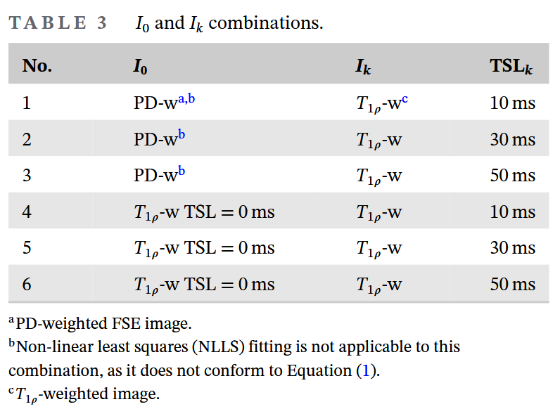
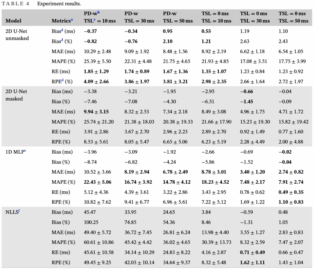
As shown in the table above, we have a total of 6 input data combinations, corresponding to the PD-w and TSL=0 T1rho images, and 3 T1rho images with non-zero TSLs. In this experiment, to exclude the influence of the model on the results, we only compare the results from the model with the lowest RPE (best performance) for each input data combination.

From this experiment, three results are evident:

• Replacing one of the data points from a T1rho image to a PD-w image does significantly affect the neural network’s performance.
• Even when one data point is a PD-w image, i.e., the 3rd, 4th, and 5th columns in Table 4 of the original paper, the neural network method can still achieve good T1rho prediction performance.
• As the non-zero TSL data point is replaced with data having a longer TSL, it can be seen that all evaluation metrics improve.

Experiment 2: Neural Network

The two neural network models showed distinctly different performances with different data combinations. We found that for four of the six data combinations, the best model was the 2D U-Net, while for the remaining two, it was the 1D MLP.

Observing these data combinations, it’s not hard to see that three of them involved PD-w images, and the remaining one involved a T1rho image with TSL = 10ms. Since the “optimal” TSL is close to the mean T1rho value [10], and the mean T1rho in our data is approximately 45.38ms, we can consider data combination 6, i.e., two T1rho images (TSL = 0/50ms), to be the closest to the signal model. Thus, we can interpret the above phenomenon as: when more out-of-distribution (OOD) data is introduced, the performance of the 2D U-Net surpasses that of the 1D MLP, and vice versa.

Experiment 3: Masking Cartilage ROI for 2D U-Net

Whether or not non-cartilage regions are masked also affects the 2D U-Net model’s performance in relation to the input data.

We observed that for four of the six data combinations, the performance without masking was better than with masking, while the opposite was true for the remaining two. And this 4+2 combination is completely consistent with the neural network model comparison in Experiment 2 above. Therefore, we can draw a similar conclusion—masking non-cartilage regions for the 2D U-Net can effectively improve model performance in non-OOD data situations, and vice versa.

Discussion & Conclusion

From the results of the three experiments above, we can easily draw the following conclusions:

• It is feasible to replace the TSL = 0 T1rho image with a PD-w image and then use a neural network for T1rho prediction.
• Our experiments verified that both the 2D U-Net and the 1D MLP attempt to fit the T1rho signal model, which is consistent with the theory of neural networks as universal approximators. However, if the neural network is required to highly fit a specific signal model, it is necessary to reduce OOD training data and noise.
• The 2D U-Net is better able to utilize image information such as morphology and edges from MRI images to optimize T1rho prediction performance under OOD data conditions.

At the same time, we must also point out the limitations of this work:

• Our dataset is too small and its distribution is not ideal. Despite using five-fold cross-validation, 40 data points are still a huge challenge. With this amount of data, we cannot make any guarantees about the model’s transferability.
• All 40 data sets came from the same location and the same MRI scanner, lacking multi-center, multi-vendor validation.
• It still requires scanning one T1rho image to complete the prediction.

We designed such a deep learning/neural network-based method with the initial hope of using the model to mine potential implicit physical information within MRI images, and ultimately to promote the clinical application of new MRI technologies. This implicit physical information may be difficult to express with a clear model. Therefore, in this context, methods based on statistics and learning, such as deep learning, have their unique charm. Based on this line of thinking, we might be able to further extend our method to other quantitative MRI techniques, such as T2, or to deduce T1rho information from T2 information. Assuming the relevant algorithms are actively implemented, we might see the widespread popularization of quantitative imaging throughout the entire process of arthritis patient management in the near future.

Due to limited space, I have omitted many detailed steps and discussions. If you are interested, please proceed to read the paper.

References

1. Chalian M, Li X, Guermazi A, et al. The QIBA Profile for MRI-based Compositional Imaging of Knee Cartilage. Radiology. 2021;301(2):423-432. doi:10.1148/radiol.2021204587
2. Liu F, Feng L, Kijowski R. MANTIS: Model-Augmented Neural neTwork with Incoherent k-space Sampling for efficient MR parameter mapping. Magnetic Resonance in Medicine. 2019;82(1):174-188. doi:10.1002/mrm.27707
3. Huang C, Wong VWS, Chan Q, Chu WCW, Chen W. An uncertainty aided framework for learning based liver T1ρ mapping and analysis. Phys Med Biol. 2023;68(21):215019. doi:10.1088/1361-6560/ad027e
4. Huang C, Qian Y, Yu SCH, et al. Uncertainty-aware self-supervised neural network for liver T1ρ mapping with relaxation constraint. Phys Med Biol. 2022;67(22):225019. doi:10.1088/1361-6560/ac9e3e
5. Huang C, Qian Y, Hou J, et al. Breathing Freely: Self-supervised Liver T1rho Mapping from A Single T1rho-weighted Image. In: Proceedings of The 5th International Conference on Medical Imaging with Deep Learning. ; 2022. Accessed July 15, 2024. https://proceedings.mlr.press/v172/huang22a.html
6. Chen W, Chan Q, Wáng YXJ. Breath-hold black blood quantitative T1rho imaging of liver using single shot fast spin echo acquisition. Quantitative Imaging in Medicine and Surgery. 2016;6(2):16877-16177. doi:10.21037/qims.2016.04.05
7. Avants BB, Epstein CL, Grossman M, Gee JC. Symmetric diffeomorphic image registration with cross-correlation: Evaluating automated labeling of elderly and neurodegenerative brain. Medical Image Analysis. 2008;12(1):26-41. doi:10.1016/j.media.2007.06.004
8. Ronneberger O, Fischer P, Brox T. U-Net: Convolutional Networks for Biomedical Image Segmentation. Medical Image Computing and Computer-Assisted Intervention, Pt Iii. 2015;9351:234-241. doi:10.1007/978-3-319-24574-4_28
9. Zhang X, Duchemin Q, Liu* K, et al. Cramér–Rao bound-informed training of neural networks for quantitative MRI. Magnetic Resonance in Medicine. 2022;88(1):436-448. doi:10.1002/mrm.29206
10. Zibetti MVW, Sharafi A, Regatte RR. Optimization of spin-lock times in T1ρ mapping of knee cartilage: Cramér-Rao bounds versus matched sampling-fitting. Magnetic Resonance in Medicine. 2022;87(3):1418-1434. doi:10.1002/mrm.29063